
Stirling engine
A Stirling engine is a machine for converting a temperature difference into mechanical work. More formally, it’s a type of closed-cycle external combustion engine. I have a toy one from Djuino Star that I can get to run by placing it on a hot mug. (The particular geometry used in the toy, and discussed here, is called the Beta configuration.)
Here’s a neat gif from Wikipedia (credit to YK Times) showing this type of engine in operation:
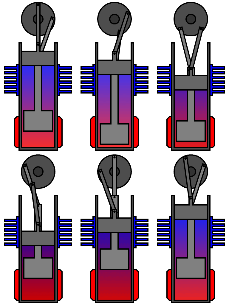
But how does it work?
Overview
Engine description
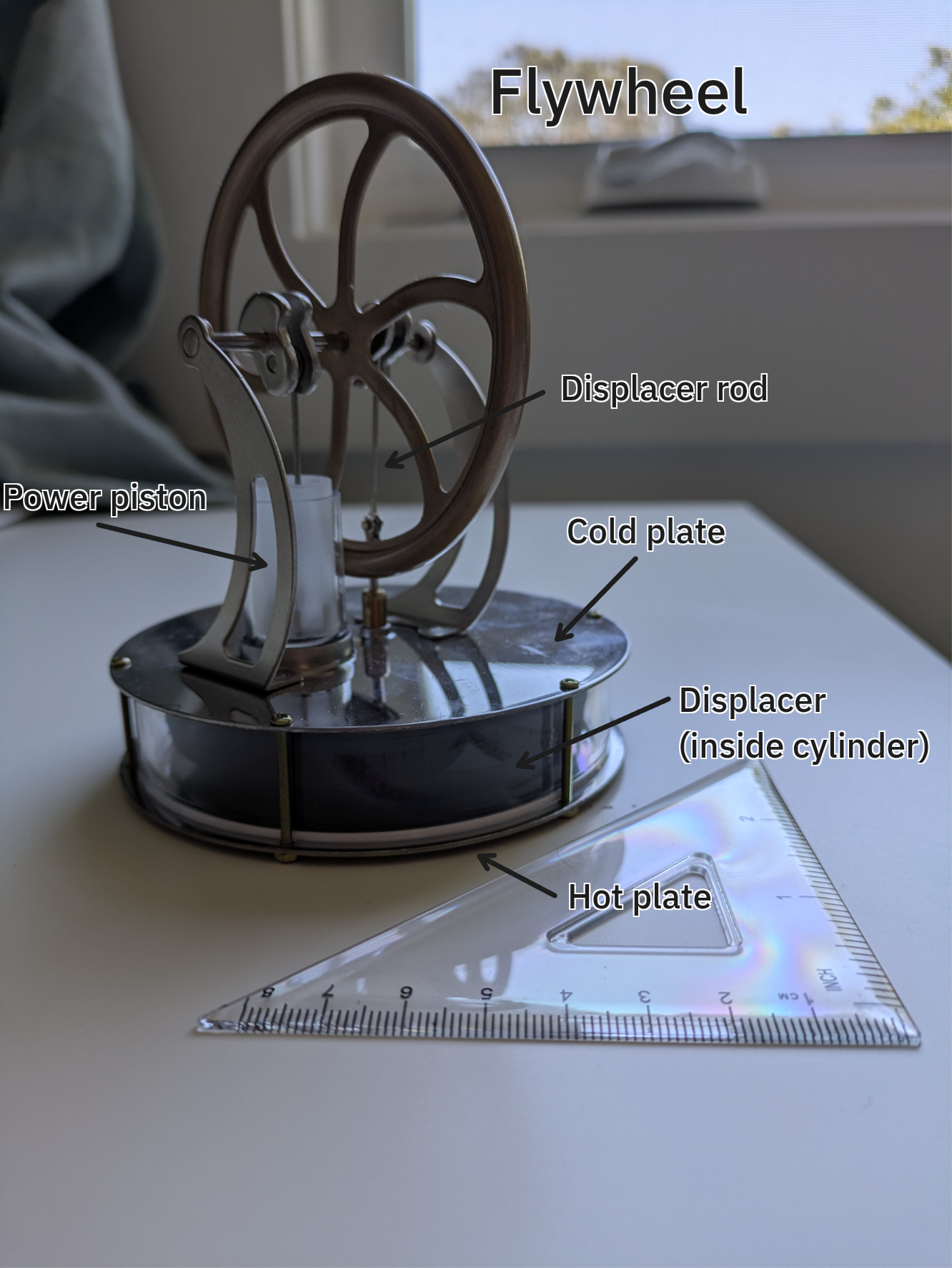
Let’s start by talking about how it’s put together. The toy engine has roughly the following parts, from bottom to top:
- A hot plate below the cylinder (e.g. a warm cup of water).
- A cylinder, wide but short.
- A displacer piston inside the cylinder. It is semi-permeable: the working gas flows freely past it. Its job is to shuttle gas between the hot (bottom) and cold (top) regions of the cylinder.
- A power piston (sealed) at the top of the cylinder. Pressure changes in the working gas push it up and down, transmitting P–V work to the flywheel.
- A large flywheel at the top. Both pistons are connected to it via crank arms that are 90° out of phase; the flywheel stores angular momentum to carry the engine through the phases where the gas torque is negative.
Note that in the actual toy engine (but not in the gif), the power piston has a much smaller radius than the displacer piston.
Thermodynamic model
The basic principle behind the engine’s operation is that the change in the internal energy of a gas associated with compression is greater at high than at low temperature. This implies that if a piston compresses a gas when the gas is cold and decompresses it when it is hot, the gas will on net do work on the piston.
The standard, simple quantitative model of this is a four-stage cycle (isothermal compression, isovolumetric heating, isothermal expansion, isovolumetric cooling; see the diagram at the link). This leads to the following estimate for the amount of work done by the engine per cycle:
\[W = n k_B \ln \frac{V_2}{V_1} (T_H - T_L)\]where \(n\) is the number of moles of the gas. This can more usefully be reexpressed as,
\[W = \frac{m}{M} k_B \ln \frac{V_2}{V_1} (T_H - T_L) \tag{1}\]where \(m\) is the mass of the gas and \(M\) the molar mass. (This form makes it clear that lighter gases, such as hydrogen and helium, lead to more powerful engines.) For a derivation, see D. Haywood, An Introduction to Stirling-Cycle Machines (pdf). Haywood also uses the differential form of the Second Law of Thermodynamics to show that the efficiency of such a four-stage cycle engine would be equal to that of the Carnot engine.
Unfortunately, the four stages of the four-stage cycle are not apparent from observing a Stirling engine in action (including the gif from Wikipedia above). The motion of the engine is clearly continuous: the sharp transitions between discrete stages are an artifact. From thermodynamics alone it is also not clear why the flywheel is needed, or how fast we expect the engine to run.
Dynamical systems model
To get a grip on these aspects, let’s try to model the Stirling engine using tools from dynamical systems theory, similarly to how I once thought about a simple DC motor.
I’ve wanted to take a stab at this for many years, but could never quite muster the energy to do so. It turns out Claude is a really delightful partner for studying problems like this, and with its help I finally made some progress!
Some interesting results:
- The PV diagram is a smooth trajectory.
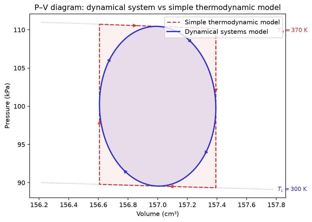
- Because the smooth PV trajectory fits within the trajectory of the thermodynamic model, the net work per cycle (equal to the area inside the closed PV curve) is less.
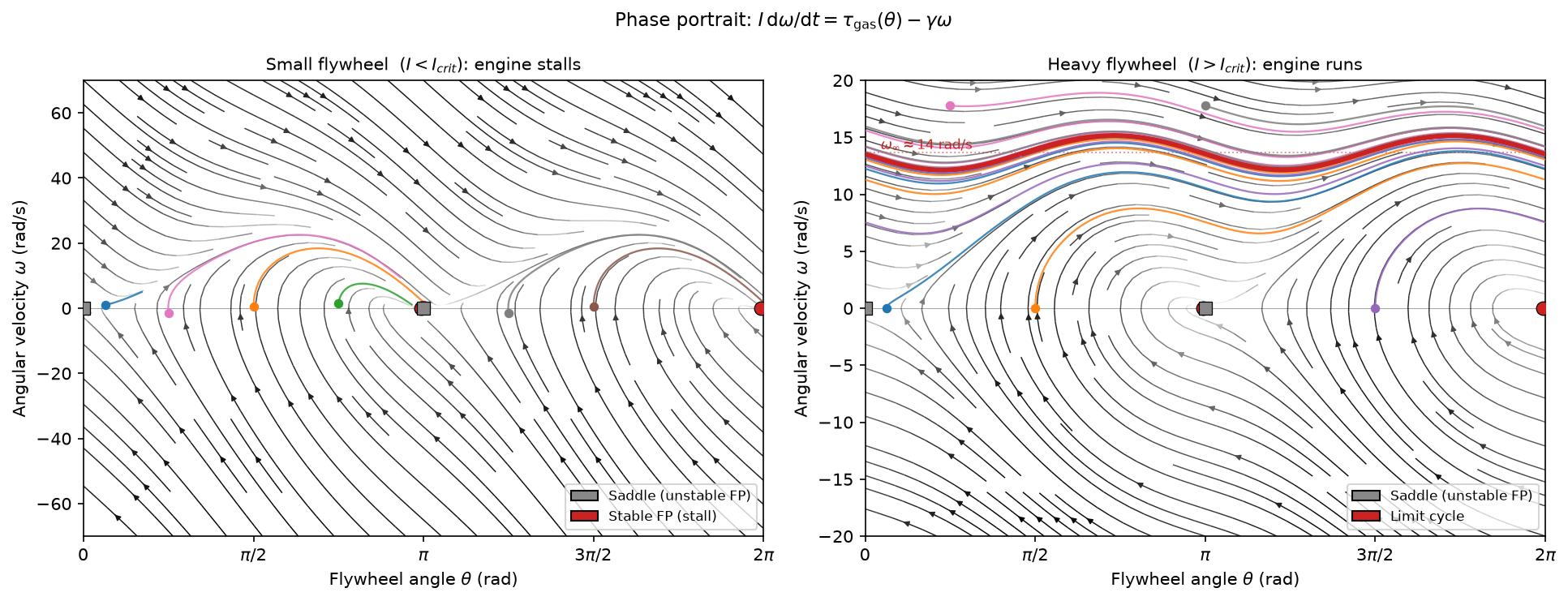
- The phase portraits show a bifurcation as the flywheel’s moment of inertia is increased. Below a critical value, the engine will come to rest before completing a single revolution. Above that value, it will spin at a roughly steady pace.
For the source code used to generate the plots below, see this repository.
Definitions and the equation of motion
In this approach, we’ll focus on two state variables: flywheel angle \(\theta\) and angular velocity \(\omega = d\theta/dt\).
Both pistons share a common crank radius \(r\), but they connect to the flywheel 90° out of phase, with the displacer leading the power piston (note this in the pictures above!):
\[x_p(\theta) = r\cos\theta, \qquad x_d(\theta) = -r\sin\theta \quad \text{(displacer leads by 90°)}\]Positive \(x_p\) means the piston moves outward (volume increases); positive \(x_d\) means the displacer is near the cold (top) end of the cylinder.
Volume (\(\varepsilon_V\))
The working gas volume is set by the power piston:
\[V(\theta) = V_0 + Ar\cos\theta\]where \(V_0\) is the dead volume (gas volume at \(\theta = \pi/2\)) and \(A\) is the piston cross-sectional area. The dimensionless ratio \(\varepsilon_V = Ar/V_0\) is the fractional volume amplitude. Note that in the toy Stirling engine, this is a small parameter: the piston has a much smaller radius than the main gas chamber.
As we’ll see below, \(\varepsilon_V\) is an important dimensionless parameter of the model.
Temperature (\(\varepsilon_T\))
The displacer controls how much gas is in contact with each plate. When \(x_d\) is positive (displacer near the cold end), the gas fills the hot region below it; when \(x_d\) is negative (displacer near the hot plate), the gas fills the cold region. The fraction of gas in the hot region is \(f_h = (1 + x_d/r)/2 = (1 - \sin\theta)/2\), giving an effective gas temperature
\[T(\theta) = T_L + \Delta T \cdot f_h = T_\text{mean} - \frac{\Delta T}{2}\sin\theta\]with \(T_\text{mean} = (T_H + T_L)/2\) and \(\Delta T = T_H - T_L\). This gives \(T = T_L\) at \(\theta = \pi/2\) (gas cold, displacer at hot end) and \(T = T_H\) at \(\theta = 3\pi/2\) (gas hot, displacer at cold end).
Another way to write this is,
\[T(\theta) = T_\text{mean}\left(1 - \varepsilon_T \sin\theta\right)\]where \(\varepsilon_T = \Delta T/(2T_\text{mean})\) is the fractional temperature amplitude. This is another important dimensionless parameter.
Pressure
Assuming ideal gas and instantaneous heat exchange (quasi-static limit):
\[P(\theta)\,V(\theta) = nRT(\theta)\]Setting mean pressure \(P_0 = nRT_\text{mean}/V_0\):
\[P(\theta) = P_0 \cdot \frac{1 - \varepsilon_T\sin\theta}{1 + \varepsilon_V\cos\theta}\]Torque and equation of motion
By virtual work, \(\tau\,d\theta = F_\text{gas}\,dx_p\), so the net torque the gas exerts on the flywheel through the power piston is
\[\tau_\text{gas}(\theta) = [P(\theta) - P_0] \cdot A \cdot \frac{dx_p}{d\theta} = -Ar\sin\theta \cdot [P(\theta) - P_0]\](\(P_\text{atm} = P_0\) balances on average; only the fluctuating part does net work.) The flywheel equation of motion is then
\[\frac{d\theta}{dt} = \omega, \qquad I\frac{d\omega}{dt} = \tau_\text{gas}(\theta) - \gamma\omega\]where \(I\) is the flywheel moment of inertia and \(\gamma\) is the viscous drag coefficient (air resistance, bearing friction, thermal losses, etc.).
A couple observations about this equation:
- It’s pretty similar to the simple DC motor equation.
- The \(-\gamma\omega\) drag term is pretty poorly motivated. Let’s keep this in mind, but go with it for now.
Net work
With the equation of motion in hand, we can do some interesting computations. For example, we can figure out the net work per cycle (the same quantity computed above for the thermodynamic model).
Substituting the pressure formula into the work integral:
\[W = \oint \tau_\text{gas}\,d\theta = ArP_0 \int_0^{2\pi} \frac{\sin\theta\,(\varepsilon_T\sin\theta + \varepsilon_V\cos\theta)}{1 + \varepsilon_V\cos\theta}\,d\theta\]The \(\varepsilon_V\) term in the numerator has the form \(\sin\theta\,f(\cos\theta)\), which is a total derivative and integrates exactly to zero over any full period (for any value of \(\varepsilon_V\)). This leaves
\[W = ArP_0\,\varepsilon_T \int_0^{2\pi} \frac{\sin^2\theta}{1 + \varepsilon_V\cos\theta}\,d\theta\]To evaluate the integral exactly, write \(\sin^2\theta = 1-\cos^2\theta\) and use the partial-fraction identity
\[\frac{\cos^2\theta}{1+a\cos\theta} = \frac{\cos\theta}{a} - \frac{1}{a^2} + \frac{1}{a^2(1+a\cos\theta)}\]together with \(\int_0^{2\pi}(1+a\cos\theta)^{-1}d\theta = 2\pi/\sqrt{1-a^2}\) to obtain
\[\int_0^{2\pi} \frac{\sin^2\theta}{1+\varepsilon_V\cos\theta}\,d\theta = \frac{2\pi\,(1-\sqrt{1-\varepsilon_V^2})}{\varepsilon_V^2}\]The closed-form result for the net work per cycle is therefore
\[W = \frac{2\pi ArP_0\,\varepsilon_T\,(1 - \sqrt{1-\varepsilon_V^2})}{\varepsilon_V^2} > 0 \quad (\Delta T > 0) \tag{2}\]This is exact in \(\varepsilon_V\) (and linear in \(\varepsilon_T\), since \(P - P_0\) is linear in \(\varepsilon_T\)).
Comparison to the thermodynamic model
At first glance, this looks very different from the expression for net work per cycle from the standard thermodynamic model (let’s call it \(W_*\)), given by Eq. 1 above:
\[W_* = \frac{m}{M} k_B \ln \frac{V_2}{V_1} (T_H - T_L)\]What is going on?
Note that (Taylor-expanding the natural logarithms),
\[W_* = \frac{m}{M} k_B \ln \frac{1 + \varepsilon_V}{1 - \varepsilon_V} (T_H - T_L) = 2 \frac{m}{M} k_B \varepsilon_V \Delta T + O(\varepsilon_V^3)\]while expanding Eq. 2 for small \(\varepsilon_V\) (fractional volume amplitude),
\[W = \pi ArP_0\,\varepsilon_T\!\left(1 + \frac{\varepsilon_V^2}{4} + O(\varepsilon_V^4)\right)\]Dropping terms higher-order in \(\varepsilon_V\),
\[W = \pi ArP_0\,\varepsilon_T = \pi A r \left(\frac{m}{M} k_B \frac{T_0}{V_0}\right)\left(\frac{\Delta T}{2 T_0}\right) = \frac{\pi}{2} \frac{m}{M} k_B \Delta T \varepsilon_V\]and so,
\[W = \frac{\pi}{4} W_* + O(\varepsilon_V^3)\]That is, to low order in \(\varepsilon_V\), our estimate of the work is exactly \(\pi/4\) of the thermodynamic model’s estimate.
The difference arises because the cycle does not consist of isothermal and isochoric sections, as assumed in the simple thermodynamic model. Instead, we’re now moving on a smooth closed trajectory in PV space.
PV diagram
Using the equations for pressure and volume as a function of \(\theta\), we can plot the PV diagram for this model, and compare it to the thermodynamic model.
Terminal angular velocity
Setting the mean driving torque \(W/(2\pi)\) equal to the drag at steady state gives the terminal angular velocity:
\[\omega_\infty \approx \frac{ArP_0\,\varepsilon_T\,(1-\sqrt{1-\varepsilon_V^2})}{\gamma\,\varepsilon_V^2}\]which reduces to \(ArP_0\Delta T/(4\gamma T_\text{mean})\) as \(\varepsilon_V \to 0\). The flywheel must have enough rotational kinetic energy to coast through the phases where \(\tau_\text{gas} < 0\); increasing \(I\) does not change \(\omega_\infty\) but widens the basin of attraction of the limit cycle.
Phase portraits
To understand the dynamics of this system, let’s examine its phase portraits: trajectories on the \((\theta, \omega)\) cylinder.
The system always has four fixed points, but the dynamics around them goes through a bifurcation as the moment of inertia increases past a critical value, \(I_\text{crit}\).
Fixed points
Fixed points satisfy \(\omega = 0\) and \(d\omega/dt = 0\), so \(\tau_\text{gas}(\theta) = 0\). Substituting the pressure formula:
\[\tau_\text{gas}(\theta) = Ar P_0 \frac{\sin\theta\,(\varepsilon_T\sin\theta + \varepsilon_V\cos\theta)}{1 + \varepsilon_V\cos\theta} = 0\]The denominator is never zero (since \(|\varepsilon_V| < 1\)), leaving two families:
-
\(\sin\theta = 0\), giving \(\theta = 0\) and \(\theta = \pi\) — the saddle points where the piston is momentarily stationary (\(dV/d\theta = 0\)).
-
\(\varepsilon_T\sin\theta + \varepsilon_V\cos\theta = 0\), i.e. \(P(\theta) = P_0\) — the stable fixed points where the gas pressure returns to its mean despite the piston still moving. This gives
whose two solutions in \((0, 2\pi)\) with \(\sin\theta \neq 0\) are
\[\theta^* = \pi - \arctan\!\frac{\varepsilon_V}{\varepsilon_T}, \qquad 2\pi - \arctan\!\frac{\varepsilon_V}{\varepsilon_T}\]Two dynamical regimes
Whether these fixed points are the final attractors depends on the flywheel inertia \(I\):
Small \(I\) (left panel, \(I < I_\text{crit}\)): The flywheel stores too little kinetic energy to coast through the braking phases of the cycle. The engine stalls: trajectories converge to one of the two stable fixed points at \(\tan\theta = -\frac{\varepsilon_V}{\varepsilon_T}\).
Large \(I\) (right panel, \(I > I_\text{crit}\)): The flywheel carries the engine through the braking regions and a stable limit cycle is born at \(\omega \approx \omega_\infty\) as an additional attractor. The stable fixed points remain stable (the linearised eigenvalues have negative real parts for all \(I > 0\)), but their basins of attraction shrink, so most initial conditions converge to the limit cycle instead. Just above \(I_\text{crit}\) the \(\omega\)-oscillation on the limit cycle is large (\(\sim 40\%\)); it shrinks as \(I\) grows.
Critical inertia
The transition between the two regimes occurs at the value \(I_\text{crit}\) for which the limit cycle is born. This is a heteroclinic bifurcation: at \(I = I_\text{crit}\), the unstable manifold of the saddle at \(\theta = 0\) connects exactly to the saddle at \(\theta = \pi\) through the upper half-plane (\(\omega > 0\)), tracing a critical orbit with \(\omega(0) = \omega(\pi) = 0\).
Exact implicit condition. Multiply the equation of motion by \(\omega\) and rewrite it as an energy equation:
\[I\frac{d(\omega^2/2)}{d\theta} = \tau_\text{gas}(\theta) - \gamma\omega\]Integrate along the critical orbit from \(\theta = 0\) to \(\theta = \pi\):
\[\underbrace{\tfrac{I}{2}\!\left[\omega(\pi)^2 - \omega(0)^2\right]}_{= \;0} = \underbrace{\int_0^\pi \tau_\text{gas}\,d\theta}_{\Phi(\pi)} \;-\; \gamma\int_0^\pi \omega^*\,d\theta\]With both endpoints at \(\omega = 0\), this gives
\[\gamma\int_0^\pi \omega^*(\theta)\,d\theta = \Phi(\pi) \equiv \int_0^\pi \tau_\text{gas}(\theta)\,d\theta\]The right-hand side, \(\Phi(\pi)\), is the net gas work over the first half-cycle; the left-hand side is the energy dissipated by drag. Because \(\omega^*\) depends on \(I\), this is an implicit condition for \(I_\text{crit}\).
Exact \(\gamma^2\) scaling. Rescale \(\omega = (\tau_0/\gamma)\hat\omega\) where \(\tau_0\) is any fixed torque scale derived from the gas cycle (e.g. the torque amplitude \(ArP_0\varepsilon_T\)). The equation of motion becomes
\[\underbrace{\frac{I\tau_0}{\gamma^2}}_{\Lambda}\;\hat\omega\,\frac{d\hat\omega}{d\theta} = \hat\tau(\theta) - \hat\omega, \qquad \hat\tau = \tau_\text{gas}/\tau_0\]The dimensionless ratio \(\Lambda \equiv I\tau_0/\gamma^2\) is the only parameter. The heteroclinic orbit condition (\(\hat\omega = 0\) at both endpoints) determines a critical value \(\Lambda_*\) that depends only on the shape of the normalized torque profile \(\hat\tau(\theta)\), which is fixed by the gas cycle and independent of \(\gamma\). Therefore \(I_\text{crit} = \Lambda_* \gamma^2/\tau_0\), and
\[\boxed{I_\text{crit} \propto \gamma^2}\]For our toy engine,
\[I_\text{crit} \approx 1.2 \times 10^{-5}\,\text{kg}\cdot \text{m}^2\]